Job vacancy, unemployment relationship clouds ‘soft landing’ prospects
Job vacancy, unemployment relationship clouds ‘soft landing’ prospects
The Federal Reserve has significantly tightened monetary policy over the past year, raising concerns that a higher unemployment rate will follow. Some economists have argued that because the job vacancy rate has been well above its prepandemic level, there is plenty of room for vacancies to fall before the unemployment rate must rise. This would allow the Fed to achieve a soft landing and avoid a recession.
We argue that a soft landing is possible but less likely than previous studies have suggested. The theoretical arguments supporting a soft landing have relied on a set of common model parameters that is inconsistent with recent empirical estimates in the academic literature.
State of the labor Market
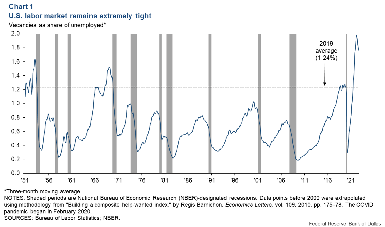
The labor market has been extremely tight. One common measure of labor market tightness is the ratio of vacancies to the number of unemployed workers (Chart 1). This measure peaked at around two vacancies for every unemployed worker in spring 2022. The ratio has since receded but remains well above 1.24 vacancies per unemployed worker observed in 2019, the year before the pandemic—at the time regarded as relatively elevated.

Elevated labor market tightness is of central concern to policymakers because it is indicative of an overheated economy and causes rapid nominal wage increases. Average hourly earnings rose about 5 percent in 2022, compared with around 3 percent in 2019. Unless accompanied by faster productivity growth, recent wage gains are likely to lead to higher prices, slowing a return to the Fed’s 2 percent annual inflation target. Throughout 2022, the 12-month PCE inflation rate exceeded 5.5 percent.
For nominal wage growth to slow to a more sustainable pace, labor market tightness must decline. This can happen through two channels: an increase in the unemployment rate (unemployed as share of the labor force), a decrease in the vacancy rate (vacancies as a share of the labor force) or a combination of the two.
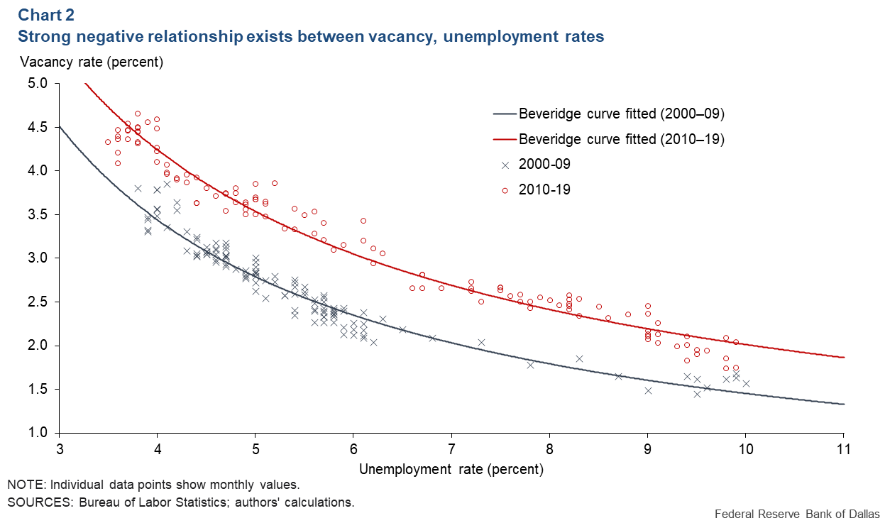
The Beveridge curve captures the relationship between vacancy and unemployment rates (Chart 2). As the vacancy rate falls, the unemployment rate rises—but less so if the vacancy rate is high. The outward shift of the Beveridge curve from the 2000s to the 2010s is due to a decline in hiring efficiency; each vacancy rate was associated with a higher unemployment rate.

During the 2000–09 and 2010–19 periods, the vacancy rate never exceeded 5 percent, well below the 2022 peak of 7.2 percent. This raises the possibility that the historical trade-off between vacancy and unemployment rates may not be a good predictor of the future.
A closer look at teh Beveridge curve matching function
While there is no historical precedent to guide expectations for how the labor market might evolve, economic theory provides insight. Consider a model of the Beveridge curve commonly used in the academic literature and the subject of a recent Feds Note article by Andrew Figura and Fed Governor Chris Waller (“What does the Beveridge curve tell us about the likelihood of a soft landing?”)
The model features three equations. The first says that workers are more likely to find jobs if there is higher rate of hiring or fewer workers competing for jobs (a lower unemployment rate). The second equation says the unemployment rate rises if layoffs increase and decreases if workers find work more easily.
The third equation is the matching function, which determines the number of hires. It states that hires increase with vacancies and unemployment but at a decreasing rate. The matching function contains three key parameters:
- Matching efficiency, which determines the number of hires for a given number of vacancies and unemployed workers. Changes in search or recruiting intensity are ways matching efficiency could change. Through the lens of this standard model, the rightward shift in the Beveridge curve in Chart 1 would correspond to declining matching efficiency.
- Matching elasticity (ε), which determines how the hiring rate changes when the number of vacancies changes. A high matching elasticity means that a small change in vacancies leads to a large change in hires, and hence a larger change in unemployment.
- Elasticity of substitution between vacancies and unemployed workers (σ) , which can take on three possible values:
- Unitary elasticity—a one-for-one relationship between the log of vacancies and unemployed workers—known as a Cobb-Douglas matching function.
- An elasticity below 1—vacancies and unemployment are gross complements.
- An elasticity above 1—vacancies and unemployment are gross substitutes.
The matching and substitution elasticities have important implications for the curvature of the Beveridge curve.
The Cobb-Douglas assumption—unitary elasticity—is the most common in the academic literature and the one used in the Feds Note article.
The gross complements assumption is an alternative sometimes appearing in the academic literature and the one used in a recent FRB San Francisco Economic Letter (“Finding a soft landing along the Beveridge curve”).
The last specification—gross substitutes—is supported by a recent empirical article by Fabian Lange and Theodore Papageorgiou (“Beyond Cobb-Douglas: flexibly estimating matching functions with unobserved matching efficiency”). This study provides the most careful and comprehensive estimates of the matching function.
Most studies use data on hires, vacancies and unemployment to estimate a log-linear version of the matching function, allowing regression analysis under the Cobb-Douglas specification. This approach prevents estimates of the degree of substitutability between vacancies and unemployment and has led to a wide range of estimates for the matching elasticity. Lange and Papageorgiou advance the literature regarding estimates of matching function parameters in two important ways. First, the authors relax the common assumption that the matching function is Cobb-Douglas. Second, they allow for multiple types of job seekers and incorporate rich measures of search effort and recruiting intensity to account for possible endogeneity—the possibility that a correlation between variables includes the effects of other factors
Insights from Theory
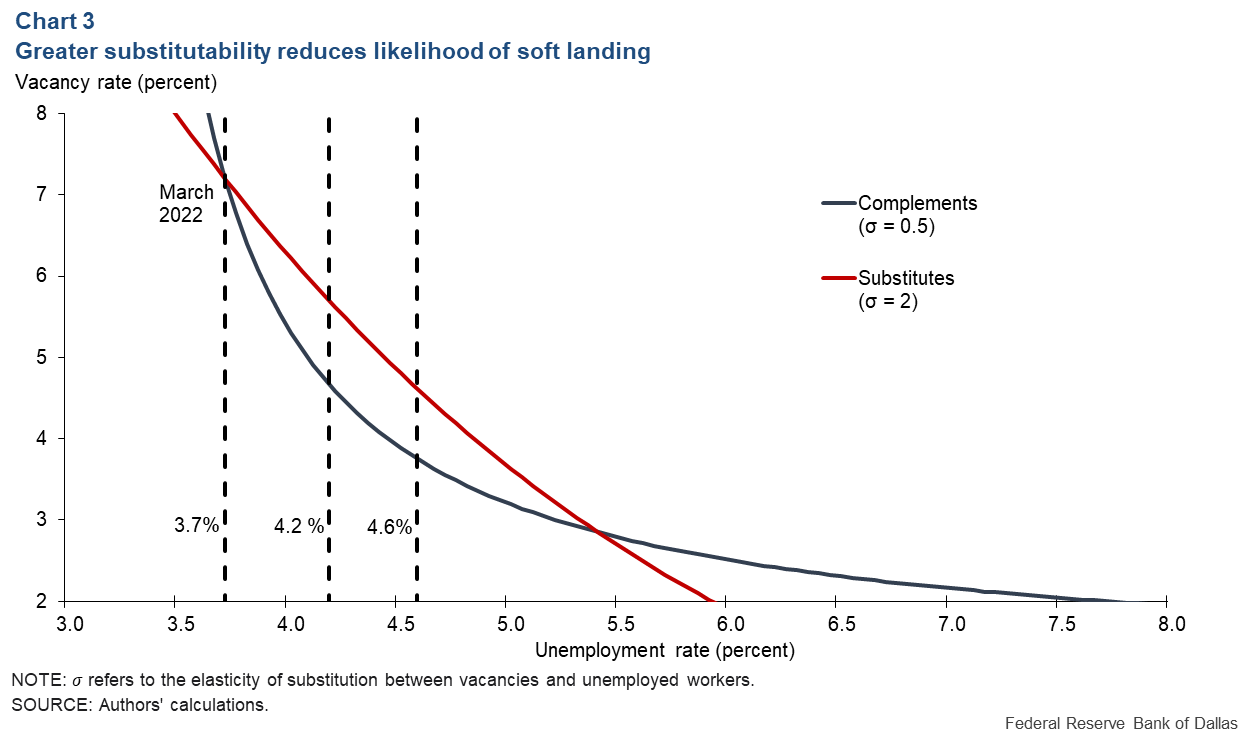
Chart 3 shows the theoretical Beveridge curve for the cases of gross substitutes (red line) and gross complements (black line), which affect how much the unemployment rate is predicted to rise for a given decrease in the vacancy rate. The matching elasticity (hiring rate changes relative to vacancies rate changes), ε, is set to 0.3, consistent with Lange’s and Papageorgiou’s estimates.

Suppose the vacancy and unemployment rates are initially equal to their March 2022 values, 7.2 and 3.7 percent, respectively, and the vacancy rate subsequently decreases to its 2019 average of 4.5 percent. If vacancies and unemployment are gross complements, then the unemployment rate increases by only 0.5 percentage points to 4.2 percent.
However, if vacancies and unemployment are gross substitutes, then unemployment increases by almost a full percentage point from the March 2022 level to 4.6 percent, above what many people would consider a soft landing. This emphasizes that a soft landing is possible under complementarity but less so under substitutability.
Of course, the change in the unemployment rate depends on the matching elasticity, which is also highly uncertain. Table 1 shows the change in the unemployment rate implied by a decline in the vacancy rate (similar to what is illustrated in Chart 3) for several parameterizations. We consider two values for the matching elasticity, ε = 0.3 and ε = 0.5. The former value is supported by Lange and Papageorgiou, while the latter specification is the most common value in the academic literature.
| Table 1: Small increases in the unemployment rate require strong assumptions | ||
| Parameterization | Complements (σ=0.5) |
Substitutes (σ=2) |
| ε=0.30, Δs=0 ε=0.50, Δs=0 |
0.5 1.0 |
0.9 2.0 |
| ε=0.30, Δs=0.25 ε=0.50, Δs=0.25 |
2.0 3.2 |
2.5 4.1 |
| ε=0.30, Δs=0.5 ε=0.50, Δs=0.5 |
3.8 6.4 |
4.0 6.3 |
| NOTE: Shown is the unemployment rate change (in percentage points) following a reduction of the vacancy rate from 7.2 percent to 4.5 percent. ε is the hiring elasticity. ∆s is the change in the layoff rate. σ refers to the elasticity of substitution between vacancies and unemployed workers. SOURCE: Authors' calculations. |
||
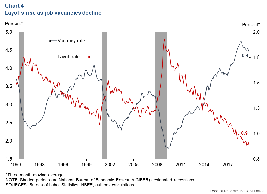
A soft landing, with the unemployment rate increasing 0.5 percentage points or less, only occurs if the matching elasticity (ε) is small, and vacancies and unemployment are gross complements. It also requires that the layoff rate does not increase. Historically, there is a negative relationship between vacancy and layoff rates (Chart 4).

If the layoff rate increases by at least 0.25 percentage points—consistent with past data—then the unemployment rate rises by at least 2 percentage points. If vacancies and unemployment are also gross substitutes, consistent with Lange and Papageorgiou, the unemployment rate rises by at least 2.5 percentage points.
Changing prospects for a soft landing
Our results suggest that a soft landing is less likely than previous articles have indicated because gross substitutability between vacancies and unemployment makes the Beveridge curve flatter—a larger change in the unemployment rate for a given change in the vacancy rate.
However, changes in matching efficiency could complicate what is observed over the next year. During the pandemic, matching efficiency likely fell due the reallocation of workers across industries.
If matching efficiency returns to its prepandemic level, it would shift the Beveridge curve left and lead to a smaller increase in the unemployment rate than Table 1 shows. In this case, reductions in demand that shift the economy along the Beveridge curve are offset by improvements in matching efficiency.


